Industrial Space Demand Forecast, First Quarter 2017

By: Dr. Joshua Harris, University of Central Florida and Dr. Hany Guirguis, Manhattan College

Despite Concerns, Industrial Space Demand Expected to Remain Strong

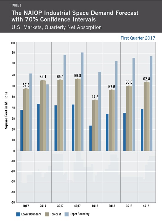
The forecast for 2017 calls for quarterly net absorption to average approximately 64 million square feet, a level similar to that realized in 2016. The model, run quarterly by Dr. Hany Guirguis, Manhattan College, and Dr. Joshua Harris, University of Central Florida, suggests that net absorption could slow to 57 million square feet per quarter in 2018 due to variation in model variables that measure GDP and unemployment. However, given uncertainty regarding federal policies and their effects on the overall economy, this figure could be revised substantially based on unforeseen events.

Overall, the consumer sector of the economy appears to be very healthy. It shows signs of steady improvement, although with some modulation in January 2017. (According to The Conference Board, consumer confidence reached a 15-year high in December 2016, but decreased slightly in January.) Hiring and wage growth remained steady from 2015 through 2016, and wealth effects from rising stock and home prices appeared to be boosting consumer spending. By pairing consumer spending with employment information, the model indicates that areas involving consumer products and e-commerce distribution are likely to remain the largest generators of demand for industrial space in 2017.

The wildcard that could cause significant growth in the U.S. economy and the industrial markets is expansion in the manufacturing and goods-producing sectors. The new Trump Administration appears to be committed to spurring growth in these fields which have in most instances, reduced production and eliminated employees since the Great Recession that took hold in 2008. This type of structural shift is not easy to predict and its impact will take time to assess. However, early indications, such as measures of business and producer confidence and future expectations included in the model, point to a higher probability of such an occurrence than at any other time since the Great Recession.

While much optimism exists among some relative to the U.S. economy, there are reasons for concern. The most palpable is the risk for higher-than-expected inflation and thus higher-than-expected interest rates. Such impacts could dampen the ability of consumers and businesses to spend and invest reducing economic activity and therefore, demand for industrial space. The risk for such an occurrence is tempering variables in the model, resulting in a net absorption forecast for 2018 that is slightly below the forecast for 2017. In reality, U.S.-based import/export markets may see some reduction in demand, while manufacturing-based markets may see a rebound. Properties providing final or “last mile” distribution to consumers will likely see gains regardless of market location.

Finally, it is worth noting that many policy stances from global trade, taxation, hiring, regulation, health care, and so forth will likely be up for debate and could change in the coming years. Changes in any of those areas could alter some of the relationships we usually see between industrial demand and the overall U.S. economy. So, as always, expect the unexpected.

Key Inputs and Disclaimers

The predictive model is funded by the NAIOP Research Foundation and was developed by Guirguis and Dr. Randy Anderson, formerly of the University of Central Florida. The model, which forecasts demand for industrial space at the national level, utilizes variables that comprise the entire supply chain and lead the demand for space, resulting in a model that is able to capture the majority of changes in demand.

While leading economic indicators have been able to forecast recessions and expansions, the indices used in this study are constructed to forecast industrial real estate demand expansions, peaks, declines and troughs. The Industrial Space Demand model was developed using the Kalman filter approach, where the regression parameters are allowed to vary with time and thus are more appropriate for an unstable industrial real estate market.

The forecast is based on a process that involves testing more than 40 economic and real estate variables that theoretically relate to demand for industrial space, including varying measures of employment, GDP, exports and imports, and air, rail and shipping data. Leading indicators that factor heavily into the model include the Federal Reserve Board’s Index of Manufacturing Output (IMO), the Purchasing Managers Index (PMI) from the Institute of Supply Management (ISM) and net absorption data from CBRE Econometric Advisors.

ISM, the Federal Reserve and CBRE Econometric Advisors assume no responsibility for the Forecast. The absorption forecast tracks with CBRE data and may vary when compared with other data sets. Data includes warehouse, distribution, manufacturing, R&D and special purpose facilities with rentable building areas of 10,000 square feet or more.

Actual versus Forecast

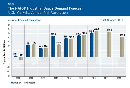
Table 2 shows actual versus forecast net absorption illustrating the model’s accurate predictive capabilities.

Initial and Ongoing Research

In 2009, the NAIOP Research Foundation awarded a research grant to Anderson and Guirguis to develop a model for forecasting net absorption of industrial space in the United States. That model led to successful forecasting two quarters out. A white paper describing the research and testing behind the model for NAIOP’s Industrial Space Demand Forecast is available at naiop.org/research.

The model was revised in 2012 to forecast eight quarters out. For this longer term forecast, Guirguis and Harris utilize the average central tendency forecast of the unemployment rate and growth rate of real GDP, provided by the seven members of the Board of Governors and the 12 presidents of the Federal Reserve Banks during the most recent Federal Open Market Committee meeting. Their forecasts are the independent variables in the equations. The forecasts usually vary from one year to another, so different techniques are applied to convert the yearly forecast to a quarterly one, in order to create the quarterly forecasts for net absorption. The estimated coefficients on the independent variables are estimated with the time-varying Kalman filter.